mdJJtest
mdJJtest Jamshidian-Jalal test for MCAR in incomplete continuous data.
Description
mdJJtest implements the diagnostic framework proposed by Jamshidian and Jalal (2010). The Hawkins, Neyman and k-sample Anderson-Darling calculations follow the modern reimplementation in function mcar of the R package mice, which is itself based on TestMCARNormality from the MissMech package. The present function is not a line-by-line reproduction of MissMech: it uses FSDA joint-normal stochastic imputation, supports multiple user-supplied completed data sets, reports median results across imputations and includes additional numerical regularization.
Example 2: Display diagnostic plots.out
=mdJJtest(Y,
Name, Value)
Examples
 Example 1: Jamshidian-Jalal test under MCAR.
Example 1: Jamshidian-Jalal test under MCAR.
rng(10)
n = 500;
p = 5;
Y = randn(n,p);
Y(rand(n,p)<0.20) = NaN;
out = mdJJtest(Y);
disp(out.pvalue)
Jamshidian-Jalal MCAR test
Retained patterns: 16
Cases used: 470 of 500
Cases removed because of sparse patterns: 30
Hawkins: median chi-square = 37.2044, df = 32, median p-value = 0.241754
No Hawkins p-value is smaller than alpha: there is no evidence against multivariate normality or MCAR.
Caution: the procedure does not distinguish MCAR from MNAR; a nonsignificant result does not rule out MNAR.

    0.2418
Example 2: Display diagnostic plots.
Example 2: Display diagnostic plots.
rng(20)
n = 600;
p = 6;
Y = randn(n,p);
Y(rand(n,p)<0.15) = NaN;
out = mdJJtest(Y,'plots',true);
Jamshidian-Jalal MCAR test
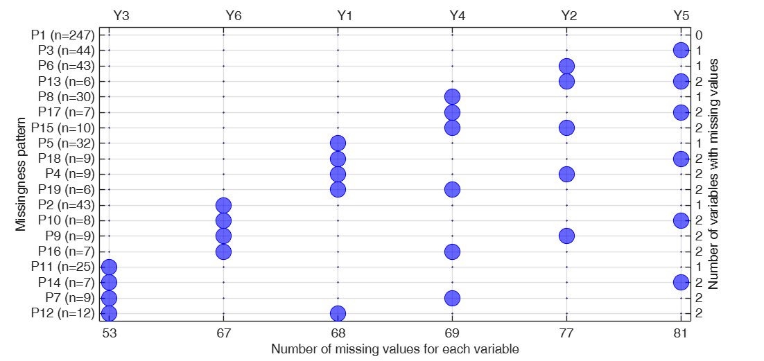
Retained patterns: 19
Cases used: 563 of 600
Cases removed because of sparse patterns: 37
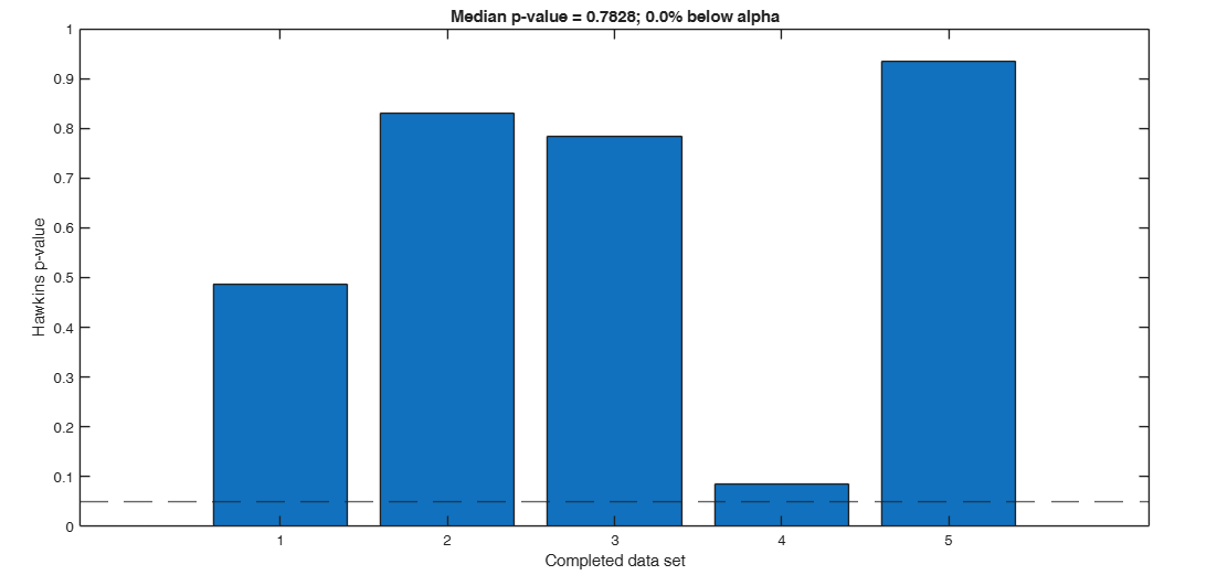
Hawkins: median chi-square = 30.9923, df = 38, median p-value = 0.78276
No Hawkins p-value is smaller than alpha: there is no evidence against multivariate normality or MCAR.
Caution: the procedure does not distinguish MCAR from MNAR; a nonsignificant result does not rule out MNAR.
Related Examples
Example 3: Use the nonparametric branch directly.
Example 3: Use the nonparametric branch directly.
rng(30)
n = 500;
p = 5;
Y = trnd(5,n,p);
Y(rand(n,p)<0.20) = NaN;
out = mdJJtest(Y,'method','nonparametric');
disp(out.ADpvalue)
Jamshidian-Jalal MCAR test
Retained patterns: 15
Cases used: 473 of 500
Cases removed because of sparse patterns: 27
Anderson-Darling: median statistic = 12.6402, median p-value = 0.591657
The Anderson-Darling rank test is not significant: there is no evidence against MCAR.
Caution: the procedure does not distinguish MCAR from MNAR; a nonsignificant result does not rule out MNAR.

    0.1672
    0.7062
    0.5114
    0.5917
    0.7428
Example 4: Supply completed data sets.
Example 4: Supply completed data sets.
rng(40)
n = 300;
p = 4;
Y = randn(n,p);
Y(rand(n,p)<0.10) = NaN;
outEM = mdEM(Y);
Yimp = cell(3,1);
for j = 1:3
Yimp{j} = mdImputeStochastic(Y,outEM.loc,outEM.cov);
end
out = mdJJtest(Y,'imputed',Yimp,'method','hawkins');
Jamshidian-Jalal MCAR test Retained patterns: 5 Cases used: 283 of 300 Cases removed because of sparse patterns: 17 Hawkins: median chi-square = 7.29487, df = 10, median p-value = 0.697345 Hawkins' test is not significant: there is no evidence against multivariate normality or MCAR. Caution: the procedure does not distinguish MCAR from MNAR; a nonsignificant result does not rule out MNAR.
Example where input is a table.
rng(50)
Y = randn(300,4);
Y(rand(size(Y))<0.15) = NaN;
Ytable = array2table(Y,'VariableNames',{'Income','Age','Score','Balance'});
out = mdJJtest(Ytable,'plots',true,'msg',false);
Input Arguments
Y — Input data.
Matrix or table.
n x p data matrix possibly containing missing values (NaN's). Rows of Y represent observations and columns represent variables.
Data Types: single | double | table
Name-Value Pair Arguments
Specify optional comma-separated pairs of Name,Value arguments.
Name is the argument name and Value
is the corresponding value. Name must appear
inside single quotes (' ').
You can specify several name and value pair arguments in any order as
Name1,Value1,...,NameN,ValueN.
 'imputed',Yimp
, 'nimputations',10
, 'minn',10
, 'method','nonparametric'
, 'nsimul',50000
, 'usechisq',50
, 'alpha',0.01
, 'maxiter',500
, 'tol',1e-8
, 'ridge',1e-8
, 'msg',false
, 'plots',true
imputed
—Completed data sets.empty value, cell array | 3D array.
If supplied, imputed can be:
(i) an n x p x M numeric array; or (ii) a cell array containing M n x p numeric matrices or tables. Observed entries should not be changed. If empty, mdEM and mdImputeStochastic are used internally.
The default value is [].
Example: 'imputed',Yimp
Data Types: double | single | cell
nimputations
—Number of stochastic imputations.positive integer.
This option is used only when imputed is empty.
The default value is 5.
Example: 'nimputations',10
Data Types: double | single
minn
—Minimum retained pattern size.integer greater than | equal to 2.
Missingness patterns containing fewer than minn observations are removed. Therefore, every retained pattern contains at least minn observations.
The default value is 6.
Example: 'minn',10
Data Types: double | single
method
—Test method.character vector | string.
Possible values are:
'auto' : Hawkins' test is computed first. If at least one Hawkins p-value is smaller than alpha, the nonparametric Anderson-Darling test is also computed;
'hawkins' : only Hawkins' test is reported;
'nonparametric' : the Anderson-Darling rank test is always reported.
The default value is 'auto'.
Example: 'method','nonparametric'
Data Types: char | string
nsimul
—Number of Monte Carlo replications used to calibrate the
fourth-order Neyman smooth test in small patterns.the default value is 10000.
Example: 'nsimul',50000
Data Types: double | single
usechisq
—Threshold for the asymptotic Neyman reference law.for a pattern containing at least usechisq observations, the chi-square approximation is used instead of Monte Carlo calibration.
The default value is 30.
Example: 'usechisq',50
Data Types: double | single
alpha
—Significance level.scalar in the interval (0,1).
The default value is 0.05.
Example: 'alpha',0.01
Data Types: double | single
maxiter
—Maximum number of iterations for mdEM.positive integer.
This option is used only when imputed is empty.
The default value is 200.
Example: 'maxiter',500
Data Types: double | single
tol
—Convergence tolerance for mdEM.positive scalar.
This option is used only when imputed is empty.
The default value is 1e-7.
Example: 'tol',1e-8
Data Types: double | single
ridge
—Numerical regularization.nonnegative scalar.
A small diagonal ridge is used to stabilize the pooled covariance matrix in Hawkins' test. The default value is 1e-10.
Example: 'ridge',1e-8
Data Types: double | single
msg
—Display test results.boolean.
If true, a concise summary is displayed.
The default value is true.
Example: 'msg',false
Data Types: logical | double
plots
—Produce graphical summaries of the diagnostic results.boolean.
The default value is false.
If plots is true, the function creates:
1) A figure containing bar charts of the available imputation-specific p-values.
If Hawkins' test is computed, the first bar chart displays the elements of $\mathtt{out.hawkinsP}$. Bar $m$ is the Hawkins p-value obtained from completed data set $m$. A horizontal reference line is drawn at alpha. The title reports the median Hawkins p-value, which is the value used as the main Hawkins result, together with the percentage of imputation-specific p-values smaller than alpha.
If the Anderson-Darling test is computed, a second bar chart displays the elements of $\mathtt{out.ADpvalue}$. Bar $m$ is the Anderson-Darling p-value obtained from completed data set $m$. A horizontal reference line is drawn at alpha. The title reports the median Anderson-Darling p-value, which is used as the main result when the Anderson-Darling branch is selected, together with the percentage of imputation-specific p-values smaller than alpha.
When both tests are available, the two bar charts are shown in separate panels of the same figure. The horizontal axis identifies the completed data sets, while the vertical axis shows the corresponding p-values.
Under method='auto', the Anderson-Darling test is activated when at least one Hawkins p-value is smaller than alpha. This activation criterion is distinct from the final decision, which is based on the median Anderson-Darling p-value when that branch is computed.
2) A graphical representation of the missingness patterns retained for the MCAR test. Rows correspond to retained missingness patterns and columns to variables.
The graphical representation is selected automatically by mdpattern. For a moderate number of patterns, a balloon plot is used: large circles denote missing entries and small filled dots denote observed entries. When the number of patterns is large, a heatmap is used, in which red cells denote missing entries and blue cells denote observed entries.
The left axis reports the frequency of each displayed pattern, while the right axis reports the number of missing variables in that pattern. Variable names are shown on the top axis and the number of missing entries for each variable is shown on the bottom axis.
Observations belonging to patterns containing fewer than minn observations are excluded before the graph is constructed. Consequently, the displayed frequencies and missing-value totals refer only to observations retained for the MCAR test.
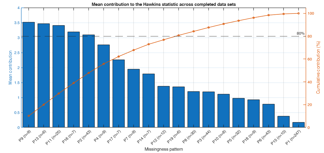
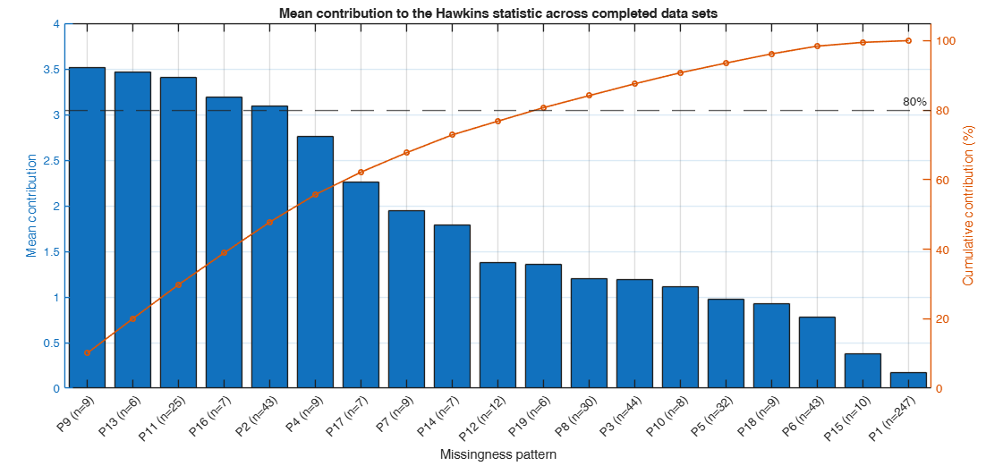
3) A Pareto plot of the mean contribution of each retained missingness pattern to every available test statistic. Contributions are first computed separately for the M completed data sets and then averaged pattern by pattern.
Bars are sorted from the largest to the smallest mean contribution. The line on the right axis reports the cumulative percentage of the total mean statistic, and a dashed horizontal line marks 80 percent. Labels such as P3 (n=12) identify the original pattern number and its frequency. These identifiers are the same as those used in the missingness-pattern figure.
Hawkins and Anderson-Darling contributions are shown in separate panels when both tests are available.
The plot is diagnostic: it reveals whether the global statistic is driven mainly by a few patterns or is distributed across many patterns.
Setting plots to false suppresses all graphical output but does not affect the numerical results returned in out.
Example: 'plots',true
Data Types: logical | double
Output Arguments
out — description
Structure
Structure containing the following fields:
| Value | Description |
|---|---|
stat |
main test statistic selected by the chosen method. If method='hawkins', or if method='auto' and the Anderson-Darling branch is not activated, out.stat is the median of the imputation-specific combined Hawkins statistics stored in $\mathtt{out.hawkinsStat}$: \[ \mathtt{out.stat} = \mathrm{median} \left\{ H^{(1)},\ldots,H^{(M)} \right\}. \] Here, $H^{(m)}$ is Fisher's combined Hawkins statistic for completed data set $m$. If method='nonparametric', or if method='auto' and the Anderson-Darling branch is activated, out.stat is the median of the imputation-specific Anderson-Darling statistics stored in $\mathtt{out.ADstat}$: \[ \mathtt{out.stat} = \mathrm{median} \left\{ A^{2(1)}_{g,n},\ldots, A^{2(M)}_{g,n} \right\}. \] Thus, out.stat is a descriptive median across completed data sets; it is not obtained using Rubin's rules or another formal multiple-imputation pooling procedure. |
pvalue |
main p-value associated with out.stat. If the Hawkins branch supplies the main result, out.pvalue is the median of the imputation-specific Hawkins p-values stored in $\mathtt{out.hawkinsP}$: \[ \mathtt{out.pvalue} = \mathrm{median} \left\{ p_{\mathrm{H}}^{(1)},\ldots, p_{\mathrm{H}}^{(M)} \right\}. \] If the Anderson-Darling branch supplies the main result, out.pvalue is the median of the imputation-specific Anderson-Darling p-values stored in $\mathtt{out.ADpvalue}$: \[ \mathtt{out.pvalue} = \mathrm{median} \left\{ p_{\mathrm{AD}}^{(1)},\ldots, p_{\mathrm{AD}}^{(M)} \right\}. \] Under method='auto', the Anderson-Darling branch is activated when at least one element of $\mathtt{out.hawkinsP}$ is smaller than alpha. Once this branch is activated, out.stat and out.pvalue are based on the Anderson-Darling results, not on the Hawkins medians. The comparison of out.pvalue with alpha gives the reported decision. The complete vectors $\mathtt{out.hawkinsP}$ and $\mathtt{out.ADpvalue}$ should also be inspected because they show the variability of the results across completed data sets. The reported median p-value is a descriptive summary and is not a formally pooled multiple-imputation p-value. |
df |
degrees of freedom of the main test. This is empty for the Anderson-Darling test; |
method |
method used; |
alpha |
significance level; |
hawkinsStat |
M x 1 vector containing the combined Hawkins statistics, one for each imputation; |
hawkinsDF |
degrees of freedom of the combined Hawkins statistic; |
hawkinsP |
M x 1 vector of Hawkins p-values; |
ADstat |
M x 1 vector of Anderson-Darling statistics, when computed; |
ADpvalue |
M x 1 vector of Anderson-Darling p-values, when computed; |
meanHawkinsContribution |
g x 1 vector containing the mean contribution of each retained missingness pattern to the Hawkins statistic across the M completed data sets. Element r is the mean of $-2\log(p_r^{(m)})$ over m. The field is empty when Hawkins' test is not computed; |
meanADContribution |
g x 1 vector containing the mean contribution of each retained missingness pattern to the Anderson-Darling statistic across the M completed data sets. The field is empty when the Anderson-Darling test is not computed; |
patterns |
g x p logical matrix containing the retained missingness patterns. A true entry denotes a missing variable; |
patternCounts |
g x 1 vector containing the frequencies of the retained missingness patterns; |
patternInfo |
table containing pattern frequency and number of missing variables. Row names identify the missingness patterns; |
npatterns |
number of retained missingness patterns; |
idxPatterns |
nused x 1 pattern membership vector; |
removedRows |
n x 1 logical vector identifying observations removed because of sparse patterns; |
removedPatterns |
matrix containing removed patterns; |
loc |
EM estimate of location used for the default stochastic imputations. Empty if imputed is supplied; |
cov |
EM estimate of covariance used for the default stochastic imputations. Empty if imputed is supplied; |
details |
cell array with detailed results for each completed data set. When Hawkins' test is computed, $\mathtt{out.details\{m\}.HawkinsContributions}$ contains the g pattern contributions for completed data set m. When the Anderson-Darling test is computed, the corresponding values are stored in $\mathtt{out.details\{m\}.AndersonDarling.}$ $\mathtt{GroupContributions}$; |
interpretation |
concise interpretation of the test; |
minn |
minimum retained pattern size. Missingness patterns containing fewer than $\mathtt{out.minn}$ observations are removed before the test is computed; |
nsimul |
number of Monte Carlo replications used to approximate the null distribution of the fourth-order Neyman smooth statistic for patterns containing fewer than $\mathtt{out.usechisq}$ observations; |
usechisq |
pattern-size threshold for the Neyman uniformity test. For a pattern containing at least $\mathtt{out.usechisq}$ observations, the asymptotic chi-square distribution with four degrees of freedom is used. For smaller patterns, Monte Carlo calibration based on $\mathtt{out.nsimul}$ replications is used; |
nimputations |
number $M$ of completed data sets analysed. This is equal to the number of stochastic imputations generated internally when imputed is empty, or to the number of completed data sets supplied through imputed; |
n |
number of observations in the original input data set, before removing observations belonging to sparse missingness patterns; |
nused |
number of observations retained and used in the test after removing observations belonging to missingness patterns containing fewer than $\mathtt{out.minn}$ observations; |
p |
number of variables in the input data set; |
More About
Additional Details
The Jamshidian-Jalal procedure assesses the MCAR assumption by comparing observations belonging to different missingness patterns. Because the test requires complete vectors, it is applied separately to each completed data set. The missingness-pattern groups are always defined using the original incomplete data.
Let a retained completed data set contain $n$ observations, $p$ variables and $g$ missingness patterns. For pattern $r$, let $n_r$ be its frequency, let $Y_{ri}$ denote completed observation $i$ in that pattern, and let
\[ \overline{Y}_r = \frac{1}{n_r}\sum_{i=1}^{n_r}Y_{ri} \]be the corresponding pattern-specific mean.
Hawkins' transformation (Hawkins, 1981) begins with the pooled within-pattern covariance matrix
\[ \widehat{\Sigma}_{P} = \frac{1}{n-g} \sum_{r=1}^{g} \sum_{i=1}^{n_r} (Y_{ri}-\overline{Y}_r) (Y_{ri}-\overline{Y}_r)^{\mathsf T}. \]Thus, variation between the pattern-specific means is removed before the common covariance matrix is estimated. Under MCAR and multivariate normality, the covariance matrices of the pattern groups should be homogeneous.
For observation $i$ in pattern $r$, the squared Mahalanobis distance from the pattern mean is
\[ d_{ri} = (Y_{ri}-\overline{Y}_r)^{\mathsf T} \widehat{\Sigma}_{P}^{-1} (Y_{ri}-\overline{Y}_r). \] Define \[ h_{ri}=n_r d_{ri}. \] Hawkins' transformation is then \[ F_{ri} = \frac{(n-g-p)h_{ri}} {p\left\{(n_r-1)(n-g)-h_{ri}\right\}}. \] Under multivariate normality and equality of the covariance matrices across missingness patterns, $F_{ri}$ has an $F$ distribution with $p$ and $n-g-p$ degrees of freedom. Consequently, the upper-tail probability \[ A_{ri} = \Pr\left\{ F_{p,n-g-p}\geq F_{ri} \right\} \]should follow a uniform distribution on $(0,1)$ within every missingness pattern.
Uniformity is assessed separately in each pattern using a fourth-order Neyman smooth test (Neyman, 1937; Rayner and Best, 1989). Let $\phi_1,\ldots,\phi_4$ denote the first four orthonormal shifted Legendre polynomials. The fourth order means that the first four components of the orthonormal polynomial expansion are retained. These components detect smooth departures from uniformity in four different directions. For pattern $r$, the statistic is
\[ N_r = \frac{1}{n_r} \sum_{\ell=1}^{4} \left\{ \sum_{i=1}^{n_r} \phi_{\ell}(A_{ri}) \right\}^{2}. \]For a pattern containing at least $\mathtt{usechisq}$ observations, $N_r$ is compared with a chi-square distribution having four degrees of freedom:
\[ N_r \mathrel{\dot{\sim}} \chi^2_4. \]
For smaller patterns, the reference distribution is approximated by generating nsimul samples of size $n_r$ from the uniform distribution and recomputing the Neyman statistic for each sample.
Let $p_r$ be the Neyman smooth-test $p$-value obtained for pattern $r$.
The pattern-specific results are combined using Fisher's method (Fisher, 1932), giving the statistic
\[ H = -2\sum_{r=1}^{g}\log(p_r). \] Under the joint null hypothesis, \[ H \mathrel{\dot{\sim}} \chi^2_{2g}. \]A small combined Hawkins $p$-value indicates that at least one pattern departs from the expected uniform behaviour. Such a rejection can be caused either by covariance heterogeneity, which provides evidence against MCAR under the assumptions of the procedure, or by departure from multivariate normality.
When method='hawkins', only this combined Hawkins test is reported. When method='auto', Hawkins' test is computed first. If at least one imputation-specific Hawkins p-value is smaller than alpha, the function also applies the k-sample Anderson-Darling test. When method='nonparametric', the Anderson-Darling test is always computed.
The k-sample Anderson-Darling test of Scholz and Stephens (1987) compares the distributions of the transformed values $F_{ri}$ across the $g$ retained missingness patterns. It extends the weighted empirical-distribution criterion introduced by Anderson and Darling (1952) to the k-sample problem. Its null hypothesis is
\[ H_0:\mathcal{F}_1=\cdots=\mathcal{F}_g, \]where $\mathcal{F}_r$ denotes the distribution of $F_{ri}$ in pattern $r$. Under MCAR, these pattern-specific distributions should be equal.
Let
\[ z_1<\cdots<z_L \]denote the distinct ordered values in the pooled sample of transformed observations, excluding the largest pooled value. For each $z_l$, let $h_l$ be its multiplicity in the pooled sample, let $H_l$ be the number of pooled observations not greater than $z_l$, and let $M_{rl}$ be the number of observations from pattern $r$ not greater than $z_l$.
The contribution of pattern $r$ to the Anderson-Darling statistic is
\[ A_r = \frac{1}{n_r} \sum_{l=1}^{L} h_l \frac{ \left(nM_{rl}-n_rH_l\right)^2 }{ H_l(n-H_l) }. \] The complete k-sample statistic is \[ A^2_{g,n} = \frac{1}{n} \sum_{r=1}^{g}A_r. \]The denominator $H_l(n-H_l)$ gives relatively high weight to distributional differences occurring in the tails. The multiplicities $h_l$ provide an adjustment for tied transformed values.
Under the null hypothesis, the expected value of $A^2_{g,n}$ is approximately $g-1$. The function computes its finite-sample variance, denoted by $\sigma^2_{g,n}$, and forms the standardized statistic
\[ T_{g,n} = \frac{ A^2_{g,n}-(g-1) }{ \sqrt{\sigma^2_{g,n}} }. \]Large positive values of $T_{g,n}$ indicate stronger differences among the pattern-specific distributions and therefore correspond to small Anderson-Darling $p$-values.
Following the approximation of Scholz and Stephens (1987), the Anderson-Darling $p$-value is not computed from a chi-square or an $F$ reference distribution. The implementation uses critical values corresponding to the five upper-tail probabilities
\[ p_l \in \{0.25,0.10,0.05,0.025,0.01\}. \]For each probability $p_l$, the corresponding critical value is approximated as a function of the number of retained patterns:
\[ q_l(g) = b_{0l} + \frac{b_{1l}}{\sqrt{g-1}} + \frac{b_{2l}}{g-1}. \]
The tabulated probabilities are transformed to log-odds:
\[ c_l = \log\left( \frac{1-p_l}{p_l} \right). \] A cubic spline interpolates the value $c$ corresponding to the observed standardized statistic $T_{g,n}$. The approximate upper-tail probability is then \[ p_{\mathrm{AD}} = \frac{1}{1+\exp(c)}. \]
Therefore, $\mathtt{out.ADpvalue}(m)$ is the approximate Anderson-Darling p-value obtained from completed data set $m$. A small value indicates that the distributions of the Hawkins-transformed quantities differ across the retained missingness patterns.
Because the calculation uses spline interpolation, and may use spline extrapolation when $T_{g,n}$ lies outside the tabulated range, very small or very large Anderson-Darling p-values should be interpreted as approximate tail probabilities.
The k-sample Anderson-Darling test is distribution free and is used to help distinguish a Hawkins rejection caused mainly by nonnormality from a rejection caused by differences among the missingness-pattern distributions. In the automatic procedure, a significant Anderson-Darling result provides evidence against MCAR within the MCAR-versus-MAR framework. A nonsignificant Anderson-Darling result following a significant Hawkins test suggests that nonnormality is the more plausible explanation.
When $M$ completed data sets are analysed, the entire procedure is repeated separately for each imputation. The imputation-specific statistics and p-values are retained in $\mathtt{out.hawkinsStat}$, $\mathtt{out.hawkinsP}$, $\mathtt{out.ADstat}$ and $\mathtt{out.ADpvalue}$.
The main reported statistic and $p$-value are the medians of the imputation-specific quantities associated with the selected branch:
\[ T_{\mathrm{reported}} = \mathop{\mathrm{median}}_{m=1,\ldots, M} T^{(m)}, \qquad p_{\mathrm{reported}} = \mathop{\mathrm{median}}_{m=1,\ldots, M} p^{(m)}. \] In particular, when the Anderson-Darling branch supplies the main result, \[ \mathtt{out.pvalue} = \mathop{\mathrm{median}} \left\{ p_{\mathrm{AD}}^{(1)},\ldots, p_{\mathrm{AD}}^{(M)} \right\}. \]
This median is a descriptive summary across imputations. It is not a Rubin-rules or Meng-Rubin pooled p-value. The complete vectors of imputation-specific p-values should therefore also be examined.
The global Hawkins and Anderson-Darling statistics can also be decomposed into nonnegative pattern-specific contributions. For Hawkins' test, let $p_r^{(m)}$ be the Neyman smooth-test p-value for retained pattern r in completed data set m. Its contribution is
\[ C_{\mathrm{H},r}^{(m)} = -2\log\left(p_r^{(m)}\right), \] and therefore \[ H^{(m)} = \sum_{r=1}^{g}C_{\mathrm{H},r}^{(m)}. \] The mean Hawkins contribution returned for pattern r is \[ \overline{C}_{\mathrm{H},r} = \frac{1}{M} \sum_{m=1}^{M} \left[-2\log\left(p_r^{(m)}\right)\right]. \] For the Anderson-Darling test, let $C_{\mathrm{AD},r}^{(m)}$ denote the normalized group contribution returned for pattern r in completed data set m. These contributions satisfy \[ A_{g,n}^{2(m)} = \sum_{r=1}^{g}C_{\mathrm{AD},r}^{(m)}, \] and their mean is \[ \overline{C}_{\mathrm{AD},r} = \frac{1}{M} \sum_{m=1}^{M}C_{\mathrm{AD},r}^{(m)}. \] Consequently, the sums of the returned mean contributions satisfy \[ \sum_{r=1}^{g}\overline{C}_{\mathrm{H},r} = \frac{1}{M}\sum_{m=1}^{M}H^{(m)}, \qquad \sum_{r=1}^{g}\overline{C}_{\mathrm{AD},r} = \frac{1}{M}\sum_{m=1}^{M}A_{g,n}^{2(m)}. \]Thus, the mean contributions decompose the mean imputation-specific statistic. They do not generally decompose $\mathtt{out.stat}$, because the latter is the median of the imputation-specific statistics.
To construct the Pareto plot, let
\[ \overline{C}_{(1)} \geq \overline{C}_{(2)} \geq \cdots \geq \overline{C}_{(g)} \] denote the mean contributions sorted from largest to smallest. The cumulative percentage after the first r sorted patterns is \[ 100 \frac{\sum_{j=1}^{r}\overline{C}_{(j)}} {\sum_{j=1}^{g}\overline{C}_{(j)}}. \]Large bars identify patterns that contribute most strongly, on average across completed data sets, to the corresponding global statistic. A large contribution is a diagnostic indication and should not be interpreted as a separate formal rejection for that pattern.
Option nsimul affects only the Monte Carlo calibration of the pattern-specific Neyman tests in the Hawkins branch. It does not affect the Anderson-Darling p-values.
When imputed is empty, mdJJtest estimates location and covariance using mdEM and generates stochastic completed data sets using mdImputeStochastic. This is a joint multivariate-normal imputation and is not identical to the default chained normal-regression imputation used by mice::mcar. To compare the MATLAB and R implementations using exactly the same completed data sets, supply them through option imputed.
The procedure addresses the MCAR-versus-MAR framework. It cannot distinguish MCAR from MNAR. Consequently, a nonsignificant result does not establish MCAR and does not rule out an MNAR mechanism.
References
Anderson, T. W. and Darling, D. A. (1952), "Asymptotic Theory of Certain Goodness-of-Fit Criteria Based on Stochastic Processes", The Annals of Mathematical Statistics, Vol. 23, No. 2, pp. 193-212.
DOI: 10.1214/aoms/1177729437.
Fisher, R. A. (1932), "Statistical Methods for Research Workers", 4th ed., Oliver and Boyd, Edinburgh.
Hawkins, D. M. (1981), "A New Test for Multivariate Normality and Homoscedasticity", Technometrics, Vol. 23, No. 1, pp. 105-110.
DOI: 10.1080/00401706.1981.10486244.
Jamshidian, M. and Jalal, S. (2010), "Tests of Homoscedasticity, Normality, and Missing Completely at Random for Incomplete Multivariate Data", Psychometrika, Vol. 75, pp. 649-674.
Jamshidian, M., Jalal, S. and Jansen, C. (2014), "MissMech: An R Package for Testing Homoscedasticity, Multivariate Normality, and Missing
Neyman, J. (1937), "'Smooth' Test for Goodness of Fit", Skandinavisk Aktuarietidskrift, Vol. 20, pp. 149-199.
Rayner, J. C. W. and Best, D. J. (1989), "Smooth Tests of Goodness of Fit", Oxford University Press, New York.
Scholz, F. W. and Stephens, M. A. (1987), "K-Sample Anderson-Darling Tests", Journal of the American Statistical Association, Vol. 82, No. 399, pp. 918-924.
DOI: 10.1080/01621459.1987.10478517.
Van Buuren, S. and Groothuis-Oudshoorn, K. (2011), "mice: Multivariate Imputation by Chained Equations in R", Journal of Statistical Software, Vol. 45, No. 3, pp. 1-67. DOI: 10.18637/jss.v045.i03.