mdMAARtest

mdMAARtest Diagnostic tests for Missing Always At Random (MAAR)

Syntax

Description

mdMAARtest implements the three diagnostic procedures proposed by Bojinov, Pillai and Rubin (2020) for investigating whether partially observed variables are associated with missingness indicators after conditioning on the fully observed variables.

The available procedures are:

1) 'ccm': comparison of conditional means;

2) 'dtmm': direct test of a postulated missingness mechanism;

3) 'cop': semiparametric Gaussian-copula diagnostic.

The null hypothesis is that the restrictions implied by MAAR, row exchangeability and conditional independence of the missingness indicators are compatible with the observed data. Rejection indicates that at least one of these assumptions is violated. The procedures are diagnostic tools and do not establish that a nonrejected mechanism is MAAR.

example

out =mdMAARtest(Y) Example 1: MAAR data and comparison of conditional means.

example

out =mdMAARtest(Y, Name, Value) Example 2: Violation of MAAR detected by conditional means.

Examples

expand all

  • Example 1: MAAR data and comparison of conditional means.
  • .

    rng(1)
    n = 500;
    p = 5;
    Yfull = randn(n,p);
    eta = -1 + Yfull(:,4) - Yfull(:,5);
    prob = 1./(1+exp(-eta));
    Y = Yfull;
    for j = 1:3
    Y(rand(n,1)<prob,j) = NaN;
    end
    out = mdMAARtest(Y,'method','ccm','plots',true);
    disp(out.pvalue)
    MAAR diagnostic: CCM
    Observations: 500; variables: 5; partially observed variables: 3
    Nominal alpha: 0.05; component alpha: 0.008333
    Overall rejection: false
    No missingness indicator was implicated.
    The diagnostic does not reject the restrictions implied by MAAR. This result does not prove that the mechanism is MAAR.
    
        1.0000    0.1619    0.2655
        0.4202    1.0000    0.1393
        0.0925    0.8767    1.0000
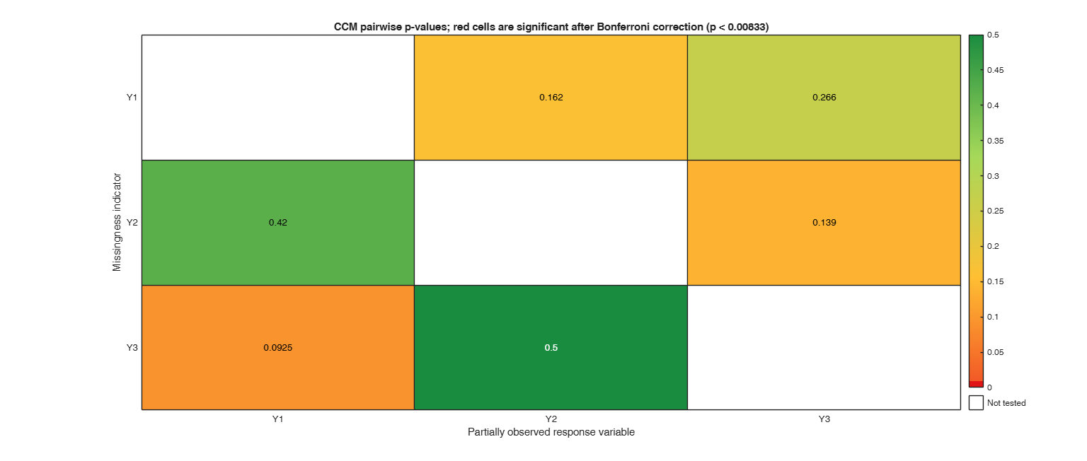
    
    
    Click here for the graphical output of this example (link to Ro.S.A. website).

  • Example 2: Violation of MAAR detected by conditional means.
  • .

    rng(2)
    n = 800;
    Yfull = randn(n,5);
    Y = Yfull;
    p1 = 1./(1+exp(-(-1+Yfull(:,4)-Yfull(:,5))));
    R1 = rand(n,1)<p1;
    p2 = 1./(1+exp(-(-1+1.5*Yfull(:,1)+Yfull(:,4)-Yfull(:,5))));
    R2 = rand(n,1)<p2;
    p3 = 1./(1+exp(-(-1+Yfull(:,1)+Yfull(:,2)+Yfull(:,4)-Yfull(:,5))));
    R3 = rand(n,1)<p3;
    Y(R1,1)=NaN; Y(R2,2)=NaN; Y(R3,3)=NaN;
    out = mdMAARtest(Y,'method','ccm','plots',true);
    disp(out.whichReject)
    MAAR diagnostic: CCM
    Observations: 800; variables: 5; partially observed variables: 3
    Nominal alpha: 0.05; component alpha: 0.008333
    Overall rejection: true
    Implicated variable indices: [2 3]
    The diagnostic rejects the restrictions implied by MAAR. Missingness indicators associated with variables [2 3] are implicated.
    
       0
       1
       1
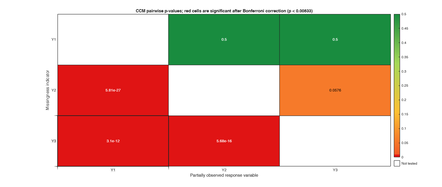
    
    
    Click here for the graphical output of this example (link to Ro.S.A. website).

    Related Examples

    expand all

  • Example 3: Direct test with multiple stochastic imputations.
  • rng(3)
       n = 500;
       Yfull = randn(n,5);
       Y = Yfull;
       pr = 1./(1+exp(-(-1+Yfull(:,4)-Yfull(:,5))));
       for j=1:3
           Y(rand(n,1)<pr,j)=NaN;
       end
       out = mdMAARtest(Y,'method','dtmm','nimputations',10);
       disp(out.DLtable)
    MAAR diagnostic: DTMM
    Observations: 500; variables: 5; partially observed variables: 3
    Nominal alpha: 0.05; component alpha: 0.01667
    Overall rejection: false
    No missingness indicator was implicated.
    The diagnostic does not reject the restrictions implied by MAAR. This result does not prove that the mechanism is MAAR.
    
                dL        rL         DL       pvalue 
              ______    _______    _______    _______
    
        Y1    3.3337    0.50166    0.74001     0.5294
        Y2    2.1112    0.57558    0.44665    0.72001
        Y3    2.4806    0.39361    0.59333    0.61987


  • Example 4: Gaussian-copula diagnostic.
  • A small number of iterations is used only to keep the example fast.

    rng(4)
       n = 300;
       Yfull = randn(n,5);
       Y = Yfull;
       pr = 1./(1+exp(-(-1+Yfull(:,4)-Yfull(:,5))));
       for j=1:3
           Y(rand(n,1)<pr,j)=NaN;
       end
       out = mdMAARtest(Y,'method','cop','niterMCMC',600,'nburnMCMC',200, ...
           'plots',true);
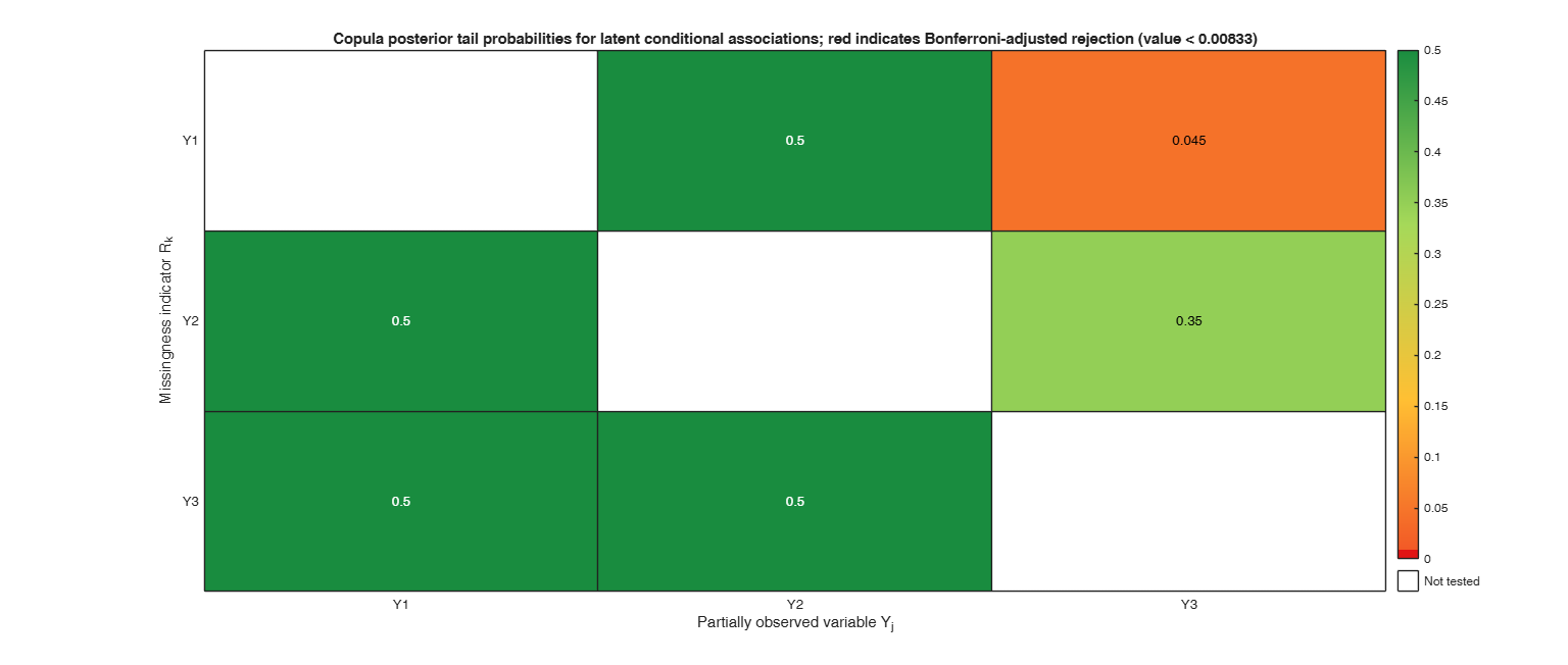
       disp(out.posteriorMedian)
    mdMAARtest copula sampler: 10% completed.
    mdMAARtest copula sampler: 20% completed.
    mdMAARtest copula sampler: 30% completed.
    mdMAARtest copula sampler: 40% completed.
    mdMAARtest copula sampler: 50% completed.
    mdMAARtest copula sampler: 60% completed.
    mdMAARtest copula sampler: 70% completed.
    mdMAARtest copula sampler: 80% completed.
    mdMAARtest copula sampler: 90% completed.
    mdMAARtest copula sampler: 100% completed.
    
    MAAR diagnostic: COP
    Observations: 300; variables: 5; partially observed variables: 3
    Nominal alpha: 0.05; component alpha: 0.008333
    Overall rejection: false
    No missingness indicator was implicated.
    The diagnostic does not reject the restrictions implied by MAAR. This result does not prove that the mechanism is MAAR.
    
        0.0647    0.0177    0.1436
       -0.0558    0.0041    0.0671
       -0.0066   -0.0501    0.0569
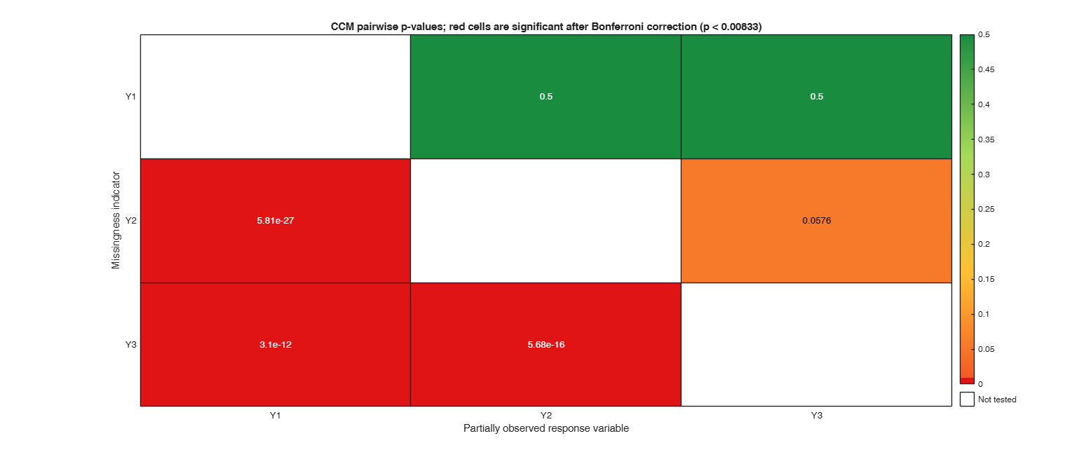
    
    
    Click here for the graphical output of this example (link to Ro.S.A. website)

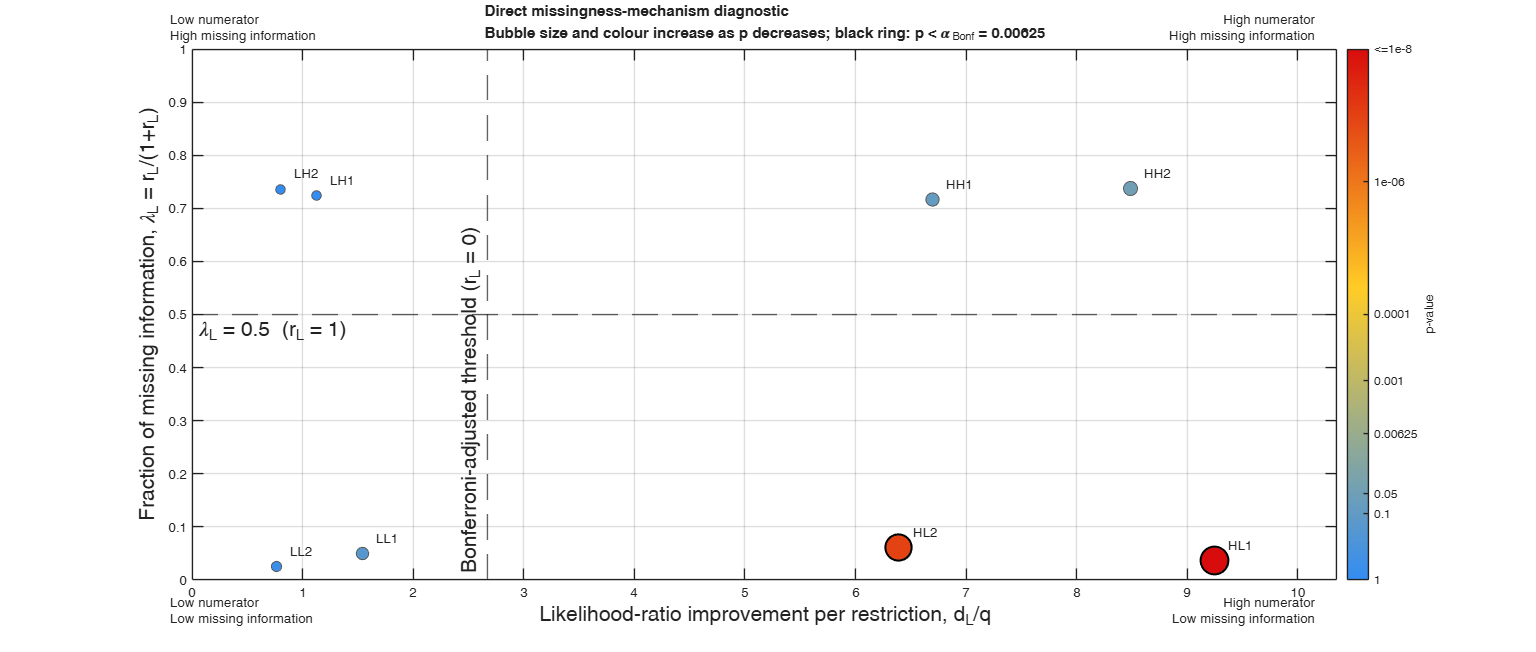
  • Complex DTMM example: variables in all four diagnostic quadrants.
  • rng(24680)
        
        n = 2500;
        q = 8;
        M = 4;
        
        % Two fully observed variables.
        X1 = randn(n,1);
        X2 = randn(n,1);
        
        % Eight variables that will contain missing values.
        Z = randn(n,q);
        
        % Complete data before introducing missing values.
        Ycomplete = [Z X1 X2];
        
        % Eight different missingness mechanisms.
        %
        % Variables 1-2:
        %   Missingness depends only on fully observed variables.
        %   Expected: low numerator, low missing information.
        %
        % Variables 3-4:
        %   Missingness additionally depends on another partially observed
        %   variable, but imputations will be very stable.
        %   Expected: high numerator, low missing information.
        %
        % Variables 5-6:
        %   No systematic dependence on partially observed variables, but
        %   imputations will deliberately disagree across completed data sets.
        %   Expected: low numerator, high missing information.
        %
        % Variables 7-8:
        %   Missingness depends on another partially observed variable and
        %   imputations will deliberately disagree.
        %   Expected: high numerator, high missing information.
        %
        % The simulation is designed to populate the four regions of the DTMM
        % diagnostic plot.
        %
        % LL1 and LL2 have a small likelihood-ratio numerator and stable
        % imputations. They are therefore expected in the lower-left region.
        %
        % HL1 and HL2 have a systematic dependence of missingness on partially
        % observed variables, producing a large numerator, while their imputations
        % are stable. They are therefore expected in the lower-right region.
        %
        % LH1 and LH2 have little systematic evidence in the numerator but their
        % imputation-specific fits disagree strongly. They are therefore expected
        % in the upper-left region.
        %
        % HH1 and HH2 combine a systematic missingness signal with substantial
        % disagreement among imputations. They are therefore expected in the
        % upper-right region.
        %
        % Importantly, the position of a point relative to the vertical reference
        % line is not by itself the final test decision. The final D_L statistic
        % also accounts for the missing-information component r_L.
        %
        % The comparison between HL and HH variables illustrates the role of r_L.
        % Both groups can have large values of d_L/q, but the HH variables have
        % much larger missing-information fractions. Consequently, their final
        % D_L statistics can be appreciably smaller and their p-values larger.
        %
        % Conversely, the LH variables show that a large missing-information
        % fraction alone does not produce rejection when the numerator contains
        % little evidence against the reduced missingness model.
        eta = zeros(n,q);
        
        % Low numerator / low missing information.
        eta(:,1) = -1.5 + 1.1*X1;
        eta(:,2) = -1.5 - 1.1*X2;
        
        % High numerator / low missing information.
        eta(:,3) = -1.0 + 0.35*Z(:,1) + 0.2*X1;
        eta(:,4) = -1.0 + 0.35*Z(:,2) - 0.2*X2;
        
        % Low numerator / high missing information.
        % These mechanisms are MCAR relative to all variables.
        eta(:,5) = 0;
        eta(:,6) = 0;
        
        % High numerator / high missing information.
        eta(:,7) = -0.5 + 0.35*Z(:,3) + 0.2*X1;
        eta(:,8) = -0.5 + 0.35*Z(:,4) - 0.2*X2;
        
        prob = 1./(1+exp(-eta));
        R = rand(n,q) < prob;
        
        % Introduce missing values.
        Y = Ycomplete;
        for j = 1:q
            Y(R(:,j),j) = NaN;
        end
        
        % Add informative variable names.
        varNames = {'LL1','LL2', ...
            'HL1','HL2', ...
            'LH1','LH2', ...
            'HH1','HH2', ...
            'X1','X2'};
        
        Y = array2table(Y,'VariableNames',varNames);
        
        % Construct four completed data sets.
        
        Imputations = cell(M,1);
        
        % Alternating signs are used to generate conflicting imputations for
        % variables 5-8.
        signImp = [-1 1 -1 1];
        
        % Small perturbation for stable imputations.
        stableNoise = 0.03;
        
        % Parameters controlling disagreement among unstable imputations.
        shift = 0.15;
        unstableNoise = 0.35;
        
        for m = 1:M
        
            % Start from the known complete simulated data.
            Ym = Ycomplete;
        
            % Variables 1-4: very stable imputations.
            for j = 1:4
                idx = R(:,j);
        
                Ym(idx,j) = Z(idx,j) + ...
                    stableNoise*randn(sum(idx),1);
            end
        
            % Variables 5-8: deliberately conflicting imputations.
            %
            % The sign of the shift reverses across imputations. Consequently,
            % the imputation-specific logistic coefficients can disagree strongly,
            % increasing r_L.
            for j = 5:8
                idx = R(:,j);
        
                Ym(idx,j) = Z(idx,j) + ...
                    signImp(m)*shift + ...
                    unstableNoise*randn(sum(idx),1);
            end
        
            Imputations{m} = Ym;
        end
        
        %Run DTMM and produce the diagnostic plot.
        out = mdMAARtest(Y,'method','dtmm', ...
            'imputed',Imputations, ...
            'plots',true, ...
            'msg',true);
    MAAR diagnostic: DTMM
    Observations: 2500; variables: 10; partially observed variables: 8
    Nominal alpha: 0.05; component alpha: 0.00625
    Overall rejection: true
    Implicated variable indices: [3 4]
    The diagnostic rejects the restrictions implied by MAAR. Missingness indicators associated with variables [3 4] are implicated.
    
    
    Click here for the graphical output of this example (link to Ro.S.A. website)

    Input Arguments

    expand all

    Y — Input data. Matrix, table or timetable.

    n x p data matrix possibly containing NaN values. Rows of Y represent observations and columns represent variables.

    Data Types: single | double | table | timetable

    Name-Value Pair Arguments

    Specify optional comma-separated pairs of Name,Value arguments. Name is the argument name and Value is the corresponding value. Name must appear inside single quotes (' '). You can specify several name and value pair arguments in any order as Name1,Value1,...,NameN,ValueN.

    Example: 'method','cop' , 'alpha',0.01 , 'ridge',1e-6 , 'msg',false , 'plots',true , 'imputed',{Yimp1,Yimp2,Yimp3} , 'nimputations',20 , 'maxiter',200 , 'tol',1e-8 , 'niterMCMC',5000 , 'nburnMCMC',1000 , 'thinMCMC',5 , 'pluginthreshold',50 , 'savesamples',true

    method —Diagnostic method.character | string.

    Possible values are:

    'ccm' = comparison of conditional means;

    'dtmm' = direct test of the missingness mechanism;

    'cop' = Gaussian-copula diagnostic.

    The default value is 'ccm'.

    Example: 'method','cop'

    Data Types: char | string

    alpha —Significance level.scalar in the interval (0,1).

    Bonferroni corrections are applied internally to the component tests. The default value is 0.05.

    Example: 'alpha',0.01

    Data Types: single | double

    msg —Display a summary of the results.boolean.

    The default value is true.

    Example: 'msg',false

    Data Types: logical | single | double

    plots —Produce a method-specific diagnostic plot.boolean.

    The default value is false.

    See More About for details. The default is false.

    Example: 'plots',true

    Data Types: logical | single | double Options used only by method 'dtmm':

    imputed —Completed data sets used by method 'dtmm'.cell array | n x p x M numeric array.

    Each completed data set must have the same dimensions as Y and must contain no missing values.

    If empty, mdEM and mdImputeStochastic are used to generate the imputations. The default value is [].

    Example: 'imputed',{Yimp1,Yimp2,Yimp3}

    Data Types: cell | single | double

    nimputations —Number of stochastic imputations for method 'dtmm' when option imputed is empty.positive integer greater than 1.

    The default value is 10.

    Example: 'nimputations',20

    Data Types: single | double

    maxiter —Maximum number of iterations passed to mdEM when imputations must be generated and to the logistic-regression fitting algorithm .the default value is 100.

    This option is used just by method 'dtmm'.

    Example: 'maxiter',200

    Data Types: single | double

    tol —Convergence tolerance passed to mdEM when imputations must be generated and to the logistic-regression fitting algorithm.the default value is 1e-5.

    This option is used just by method 'dtmm'.

    Example: 'tol',1e-8

    Data Types: single | double Options used only by method 'cop':

    niterMCMC —Number of MCMC iterations for method 'cop'.the default value is 2000.

    Example: 'niterMCMC',5000

    Data Types: single | double

    nburnMCMC —Number of initial MCMC iterations discarded for method 'cop'.the default value is 500.

    Example: 'nburnMCMC',1000

    Data Types: single | double

    thinMCMC —MCMC thinning interval for method 'cop'.the default value is 1.

    Example: 'thinMCMC',5

    Data Types: single | double

    pluginthreshold —Threshold used by the Gaussian-copula sampler.margins having more than pluginthreshold distinct observed values use fixed normal scores, as in sbgcop.

    The default value is 100 (this option is used just by method 'cop').

    Example: 'pluginthreshold',50

    Data Types: single | double

    savesamples —Save the posterior conditional-covariance draws produced by method 'cop'.boolean.

    The default value is false (this option is used just by method 'cop').

    Example: 'savesamples',true

    Data Types: logical | single | double

    Output Arguments

    expand all

    out — description Structure

    Structure containing the following fields:

    Value Description
    method

    selected diagnostic method.

    reject

    true if at least one component test rejects.

    whichReject

    logical vector associated with the variables containing missing values. Element k is true when the missingness indicator of that variable is implicated by the diagnostic.

    pvalue

    component significance measures.

    For methods 'ccm' and 'cop', out.pvalue is a q-by-q matrix, where q is the number of partially observed variables. Rows correspond to missingness indicators $R_i$ and columns to partially observed variables $Y_j$.

    For method 'ccm', out.pvalue(i,j) is the p-value of the nested-model F test comparing the conditional mean of $Y_j$ across the groups defined by $R_i$, after conditioning on the fully observed variables. A small value indicates that knowing whether variable i is missing provides additional information about the conditional mean of $Y_j$. Diagonal elements are not tested.

    For method 'cop', out.pvalue(i,j) is the two-sided posterior tail probability for the latent conditional covariance between missingness indicator $R_i$ and partially observed variable $Y_j$, given the fully observed variables. A small value indicates that most posterior mass lies on one side of zero. These quantities are posterior tail probabilities, not classical frequentist p-values. Diagonal elements are not tested.

    For method 'dtmm', out.pvalue is a q-by-1 vector. Element out.pvalue(i) is the pooled Meng-Rubin $D_L$ p-value for the missingness mechanism of variable i. It compares a reduced logistic model for $R_i$ containing only fully observed variables with a full model that also contains all imputed partially observed variables. A small value indicates that at least one partially observed variable provides additional information about whether variable i is missing.

    stat

    method-specific test statistics.

    alpha

    nominal significance level.

    alphaAdjusted

    Bonferroni-adjusted component level.

    missingVariables

    indices of variables containing NaNs.

    fullyObservedVariables

    indices of fully observed variables.

    variableNames

    variable names.

    missingIndicator

    n x q matrix; 1 denotes a missing value.

    n

    number of observations.

    p

    number of variables.

    nvarmiss

    number q of partially observed variables.

    interpretation

    concise interpretation of the result.

    Additional fields for method 'ccm':

    out.df1,

    df2

    degrees of freedom of the nested-model F tests.

    rejectPairs

    q x q logical matrix of rejected comparisons.

    Additional fields for method 'dtmm':

    out.df1, out.df2 = D_L reference-distribution degrees of freedom.

    relativeIncrease

    relative increase in variance due to nonresponse in the pooled likelihood-ratio test.

    DLtable

    table with one row for each partially observed variable and columns dL, rL, DL and pvalue.

    Row names are the corresponding variable names.

    deviance

    detailed deviances used in the D_L calculation.

    imputationInfo

    information about the completed data sets.

    Additional fields for method 'cop':

    CI

    q x q x 2 array of simultaneous credible limits.

    posteriorMean

    posterior means of conditional covariances.

    posteriorMedian

    posterior medians.

    out.rejectPairs = q x q logical matrix of rejected associations.

    nSaved

    number of retained MCMC draws.

    samples

    posterior draws when savesamples is true.

    More About

    expand all

    Additional Details

    This function implements the three diagnostics from Bojinov, Pillai and Rubin:

    $\mathbf{ccm}$: comparison of conditional means using nested Gaussian linear models and Bonferroni correction.

    $\mathbf{dtmm}$: direct testing of the missingness mechanism through logistic models and multiple imputation. The likelihood-ratio statistics are combined using the Meng-Rubin $D_L$ procedure, often referred to as the $D_3$ procedure in the multiple-imputation literature.

    ​ $\mathbf{cop}$: gaussian-copula diagnostic based on posterior conditional covariances between partially observed variables and missingness indicators.

    ---------------------------------------------------.

    $\mathbf{ccm}$ method.

    Let $J_m$ denote the set of variables that contain missing values and $J_f$ the set of fully observed variables, and let

    \[ q=|J_m| \]

    denote the number of partially observed variables. Under the assumptions considered by Bojinov, Pillai and Rubin, a missingness indicator $R_k$ should not depend on another partially observed variable $Y_j$ after conditioning on $Y_{J_f}$.

    The comparison-of-conditional-means procedure tests this implication by comparing, for every $j$ different from $k$, the nested linear models

    \[ Y_j \sim Y_{J_f} \] and \[ Y_j \sim Y_{J_f} + R_k + Y_{J_f}:R_k. \]

    $\mathbf{dtmm}$ method.

    The direct procedure (dtmm) tests the postulated missingness mechanism separately for each missingness indicator $R_k$. For a given $R_k$, the reduced logistic model contains only an intercept and the fully observed variables $Y_{J_f}$:

    \[ \mathrm{logit}\{ \Pr(R_k=1\mid Y_{J_f}) \} = \alpha_k+Y_{J_f}^{\mathsf T}\beta_k. \] The full model additionally contains all the partially observed variables after imputation. Thus, in completed data set $m$, \[ \mathrm{logit}\{ \Pr(R_k=1\mid Y_{J_f},Y_{J_m}^{(m)}) \} = \alpha_k^{(m)} +Y_{J_f}^{\mathsf T}\beta_k^{(m)} +(Y_{J_m}^{(m)})^{\mathsf T}\gamma_k^{(m)}. \]

    The response $R_k$ and the fully observed variables do not change across imputations. Consequently, the reduced model is identical in all completed data sets and is fitted only once. The full model, on the other hand, depends on the imputed values and is fitted separately in each of the $M$ completed data sets.

    Let $\widehat\theta_k^{(m)}$ denote the vector of full-model coefficient estimates obtained from completed data set $m$. The Meng-Rubin $D_L$ procedure first forms the common pooled coefficient vector

    \[ \overline\theta_k = \frac{1}{M} \sum_{m=1}^M \widehat\theta_k^{(m)}. \] Each completed data set is then reevaluated at this same pooled coefficient vector, without refitting the model. If $D_{F,m}(\widehat\theta_k^{(m)})$ is the full-model deviance evaluated at its own maximum-likelihood estimate and $D_{F,m}(\overline\theta_k)$ is the deviance evaluated at the pooled coefficients, their average difference \[ \frac{1}{M} \sum_{m=1}^M \left\{ D_{F,m}(\overline\theta_k) - D_{F,m}(\widehat\theta_k^{(m)}) \right\} \]

    measures the loss of fit caused by forcing all imputations to use a common full-model parameter vector. It therefore measures the disagreement among the imputation-specific estimates and is used to estimate the additional uncertainty due to missing information.

    Since the full model adds the $q$ partially observed variables, the estimated relative increase in variance is

    \[ r_L = \frac{M+1}{q(M-1)} \frac{1}{M} \sum_{m=1}^M \left\{ D_{F,m}(\overline\theta_k) - D_{F,m}(\widehat\theta_k^{(m)}) \right\}. \] Let $D_R$ denote the deviance of the reduced model. The numerator used by this function is \[ d_L = \max\left\{0, D_R - \frac{1}{M} \sum_{m=1}^M D_{F,m}(\overline\theta_k) \right\}. \] The maximum with zero is only a numerical safeguard against tiny negative values caused by finite-precision calculations. The pooled Meng-Rubin statistic used by this function is then \[ D_L = \frac{d_L}{q(1+r_L)}. \]

    Thus $d_L$ measures the improvement of the full model over the reduced model after imposing common pooled coefficients, whereas $r_L$ quantifies the additional uncertainty arising when the imputation-specific full-model estimates disagree substantially.

    The relative increase $r_L$ can also be expressed through the corresponding fraction of missing information,

    \[ \lambda_L=\frac{r_L}{1+r_L}. \]

    This transformation maps $r_L\in[0,\infty)$ into $\lambda_L\in[0,1)$. Values close to zero correspond to little missing-information uncertainty, whereas values approaching one correspond to a large missing-information component. The DTMM diagnostic plot therefore uses $\lambda_L$ on the vertical axis, while the original $r_L$ is reported in out.DLtable.

    The resulting statistic is compared with the finite-$M$ $F$ reference distribution of Meng and Rubin (1992).

    A small $p$-value indicates that, after conditioning on the fully observed variables, at least one partially observed variable provides additional information about the missingness indicator $R_k$.

    $\mathbf{cop}$ method.

    The Gaussian-copula procedure uses the extended rank-likelihood sampler of Hoff (2007). For every retained posterior correlation matrix, the function computes the covariance between the partially observed outcomes and their missingness indicators conditional on the fully observed variables. A component is rejected when its Bonferroni-adjusted credible interval does not contain zero.

    The original R implementation uses mice for method 'dtmm'. When option imputed is empty, this MATLAB implementation instead uses the joint-normal EM and stochastic-imputation functions already available in FSDA.

    $\large{\text{PLOTS IN OUTPUT}}$.

    If plots is true, the graphical summary depends on the selected diagnostic method:

    $\mathbf{ccm}$ Produces a q-by-q heatmap of the pairwise F-test p-values. Rows correspond to missingness indicators $R_i$ and columns to partially observed variables $Y_j$. Diagonal cells are not tested. Small p-values are shown using reddish colours, and cells significant after the Bonferroni correction are displayed in red.

    $\mathbf{dtmm}$ Produces a bubble scatter plot that separates the two components entering the Meng-Rubin $D_L$ statistic,

    \[ D_L=\frac{d_L}{q(1+r_L)}. \]

    The horizontal coordinate $d_L/q$ measures the likelihood-ratio improvement in fit per tested restriction obtained by augmenting the reduced missingness model with the partially observed variables.

    More precisely, $d_L$ is the reduction in deviance obtained by moving from the reduced model to the full model when the latter is evaluated using the common coefficient vector pooled across imputations.

    The vertical coordinate is

    \[ \lambda_L=\frac{r_L}{1+r_L}, \]

    a bounded representation of the missing-information component. There is one bubble for each missingness indicator, labelled with the corresponding variable name. Bubble size and colour increase as the associated $p$-value decreases; a black ring identifies components rejected at the Bonferroni-adjusted significance level.

    The vertical reference line is the Bonferroni-adjusted threshold for $d_L/q$ under $r_L=0$. The horizontal reference line $\lambda_L=0.5$, equivalently $r_L=1$, is an interpretative benchmark for the missing-information component. These reference lines are graphical guides; the formal decision is based on the finite-$M$ Meng-Rubin $p$-value.

    For graphical readability, numerator values exceeding six times the reference threshold are displayed at that upper bound and marked by a right-pointing symbol. Their exact values remain available in out.DLtable.

    $\mathbf{cop}$ Produces a q-by-q heatmap of the two-sided posterior tail probabilities for the latent conditional covariances between missingness indicators $R_i$ and partially observed variables $Y_j$, conditional on the fully observed variables. Rows correspond to $R_i$ and columns to $Y_j$. Diagonal cells are not tested. Small posterior tail probabilities are shown using reddish colours, and rejected components are displayed in red.

    The plot is created in a new MATLAB figure. Setting plots to false suppresses all graphical output but does not affect the numerical results returned in out.

    References

    Bojinov, I., Pillai, N. S. and Rubin, D. B. (2020), "Diagnosing missing always at random in multivariate data", Biometrika, Vol. 107, pp. 246-253.

    Hoff, P. D. (2007), "Extending the rank likelihood for semiparametric copula estimation", Annals of Applied Statistics, Vol. 1, pp. 265-283.

    Meng, X.-L. and Rubin, D. B. (1992), "Performing likelihood ratio tests with multiply-imputed data sets", Biometrika, Vol. 79, pp. 103-111.

    Bojinov, I. (2018). diagMAAR: Diagnostic tests for missing always at random [Repository GitHub], https://github.com/bojinov/diagMAAR/

    This page has been automatically generated by our routine publishFS